Sec.2-Ch.2-Subsec.7:A Practical Guide to Bayesian Diagnostic Meta-Analysis in R(II)


In medical diagnostic test research, how to effectively synthesize evidence across multiple studies while accurately quantifying the uncertainty of sensitivity and specificity has always been a core statistical challenge. Compared with traditional Meta-analysis, the Bayesian framework can naturally handle uncertainty, flexibly adapt to different data structures, and maintain robust performance in settings with small sample sizes and high heterogeneity. This article demonstrates the full analytical process with code implementation.
Review of Bayesian Meta-Analysis
In the previous article, we discussed that Bayesian Meta-analysis is an advanced data synthesis method based on Bayesian statistical principles. It significantly extends and optimizes traditional Meta-analysis. Conventional Meta-analysis typically adopts fixed-effect or random-effects models, combining effect sizes from multiple independent studies through weighted aggregation to obtain an overall effect estimate.
The fixed-effect model assumes that all studies share the same true effect, which is suitable when no substantial heterogeneity exists across studies. In contrast, the random-effects model assumes that effect sizes vary between studies, making it more appropriate for highly heterogeneous research environments.
However, in diagnostic test Meta-analysis, sensitivity and specificity are often analyzed separately, ignoring their negative correlation and between-study heterogeneity. This may lead to underestimation of true uncertainty.
Bayesian Meta-analysis adopts a fundamentally different statistical framework: it treats both data and model parameters as random variables. By combining prior distributions with the likelihood derived from observed data, posterior distributions are generated to quantify parameter uncertainty. This approach allows incorporation of expert knowledge or prior research evidence into the analysis.
Beyond synthesizing evidence from different studies, Bayesian Meta-analysis provides more transparent, robust, and generalizable conclusions—particularly under small sample or sparse data conditions. Compared with traditional approaches, it offers substantial advantages in handling heterogeneity, quantifying parameter uncertainty, model flexibility, and extrapolation capability. It is widely used in complex hierarchical models, diagnostic bivariate analyses, and network Meta-analysis.
In practical applications, the R package bamdit provides a convenient and powerful tool for Bayesian diagnostic Meta-analysis. It is based on a scale-mixture bivariate random-effects model and can integrate research data of varying types and quality, including randomized controlled trials and observational studies. It accounts for both internal and external validity bias, improving robustness.
The core function metadiag() estimates sensitivity and specificity, supporting:
Bivariate random-effects modeling
Different link functions
Evidence conflict handling
Prediction for new studies
Computation is performed via JAGS using MCMC sampling, generating full posterior distributions of parameters. This enables researchers to quantify uncertainty under small samples or high heterogeneity, rather than relying solely on point estimates and confidence intervals.
Additionally, bamdit provides Bayesian summary ROC curves, AUC calculation, visualization tools, and prior specification functions, greatly simplifying traditional Bayesian diagnostic Meta-analysis workflows and enabling clinicians and statisticians to conduct complex analyses efficiently and robustly.
1. Data Preparation
The bamdit package includes the example dataset glas from Glas et al. (2003), covering detection data for multiple biomarkers. In actual analysis, researchers typically filter for markers of interest, such as Telomerase, to ensure targeted analysis. Filtering specific markers not only reduces heterogeneity interference but also facilitates accurate estimation of sensitivity and specificity in subsequent models.
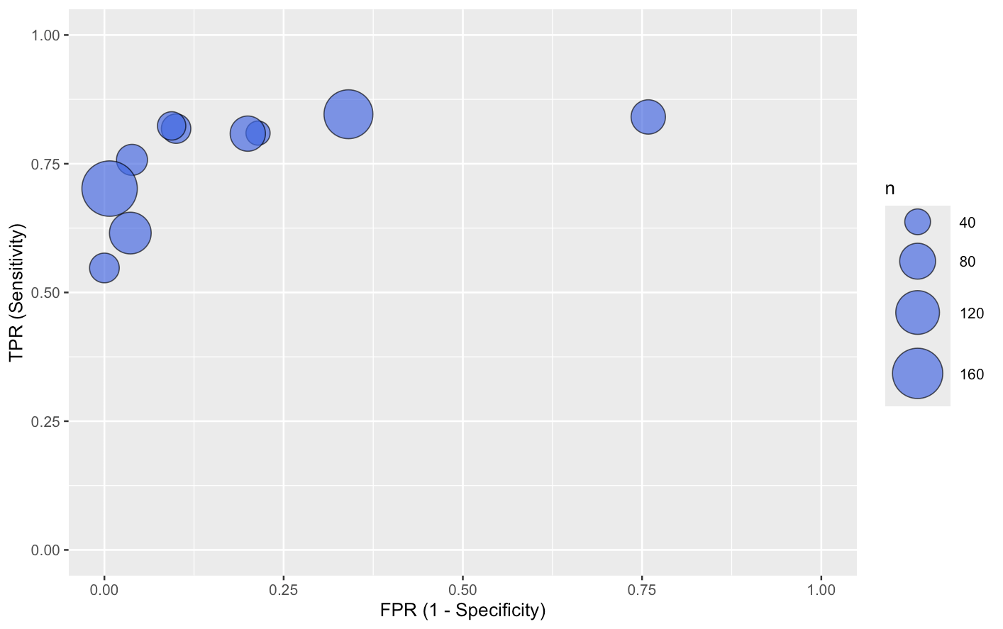
The core goal of data organization is to structure the 2×2 table information from each study into an R data frame, commonly with columns in the order: TP (True Positives), number of diseased patients (N1), FP (False Positives), and number of non-diseased patients (N2). This structure is the default reading format for the metadiag() function. During organization, attention must be paid to missing values, outliers, and sample size differences, as these factors directly affect MCMC sampling convergence and posterior distribution stability. After completing data organization, preliminary visualization is crucial. The plotdata() function can intuitively display the distribution of sensitivity and specificity for each study, helping researchers identify negative correlation patterns, outliers, and potential heterogeneity.
library(bamdit)
data("glas")

# Select data for Telomerase marker, keeping first four columns: tp, n1, fp, n2
glas.t <- glas[glas$marker == "Telomerase", 1:4]

# Visualize data distribution
plotdata(glas.t, two.by.two = FALSE)